8 Chapter 7 - Model ensemble
In this chapter, we require the 60 models resulting from the combinations of pseudo-absence sets, modeling algorithms, and resampling strategies for each species. Ensembling models involves summarizing all this information into a single prediction. This allows us to capture a wide range of possible responses arising from the different combinations. Some algorithms have a stochastic nature, like machine learning methods, and even without changing any other conditions, running the model with the same data might generate slightly different predictions. Other algorithms are more static, such as GLM: running the model with exactly the same data will generate the same prediction. That’s one reason we vary the initial conditions of the model (e.g., pseudo-absences dataset and resampling). This wider range of predictions is supposed to capture slight variations in information about the species’ niche and thus create a more robust final model.
For this chapter we will need again the biomod2 package.
8.1 Ensembling Vipera aspis
Assuming that we have a clean workspace, we have to load the models from the folder where they were saved models/vaspis. As biomod2 deals with very different algorithms and data, it saves many information and data that might be cumbersome to understand what is in the folder. However, by importing into R one of the files, we can access all information through biomod2 functions. It requires a small coding trick to fully import the model data with a common object name. We have to load and retrieve that data in two lines of code:
The object vaModel contains all the models built in the previous chapter. Now, we can proceed with ensembling. The package provides a straightforward function with customizable arguments for ensembling. We specify the models we want to ensemble and choose the type of ensembling. In this example, we are ensembling all models together, meaning that all combinations of pseudo-absences, algorithms, and runs are merged. However, we could choose to ensemble only specific subsets, such as by algorithm, by setting em.by = "PA_dataset+repet", which would result in separate ensembles for each algorithm. This approach could be useful for evaluating the performance of each algorithm individually. Here, we are ensembling all models together using em.by = "all" while models.chosen = 'all' ensures that all built models are available for ensembling.
We select the median as the ensembling statistic. Other options available include mean and weighted mean, where weights are typically based on model performance metrics or confidence intervals.
Since the resulting ensemble model provides predictions that have not yet been tested, we evaluate its performance using the same metrics as before (TSS and ROC). Variable importance is also assessed using 3 permutations, as in previous steps.
vaEnsbl <- BIOMOD_EnsembleModeling(bm.mod = vaModel,
                                   models.chosen = 'all',
                                   em.by = 'all',
                                   em.algo = 'EMmedian',
                                   metric.eval =  c('TSS', 'ROC'),
var.import = 3)##
## -=-=-=-=-=-=-=-=-=-=-=-=-= BIOMOD.ensemble.models.out -=-=-=-=-=-=-=-=-=-=-=-=-=
##
## sp.name : Vaspis
##
## expl.var.names : evi BIO_8 BIO_3 BIO_12 BIO_1
##
##
## models computed:
## Vaspis_EMmedianByTSS_mergedData_mergedRun_mergedAlgo, Vaspis_EMmedianByROC_mergedData_mergedRun_mergedAlgo
##
## models failed: none
##
## -=-=-=-=-=-=-=-=-=-=-=-=-=-=-=-=-=-=-=-=-=-=-=-=-=-=-=-=-=-=-=-=-=-=-=-=-=-=-=-=At this stage, we should have a new file in the models/Vaspis folder containing the ensembling results, which we can access later as needed.
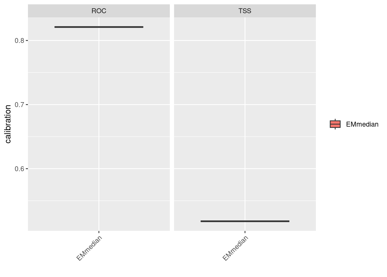
We can evaluate the ensembled model by plotting its performance metrics. Now we don’t have calibration and validation datasets and we test with full data.
Both metrics show reasonable performance. However, at this stage, we should consider adding more predictors or potentially removing some to improve model performance. If an important predictor defining the species niche is missing, it could significantly affect performance. Another strategy could involve adjusting the width of the buffer for pseudo-absences. Increasing environmental variability might facilitate model fitting, but this approach should be carefully balanced and justified (as it might be a contentious subject!).
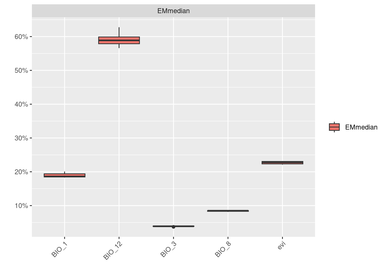
We can also check the variable importance.
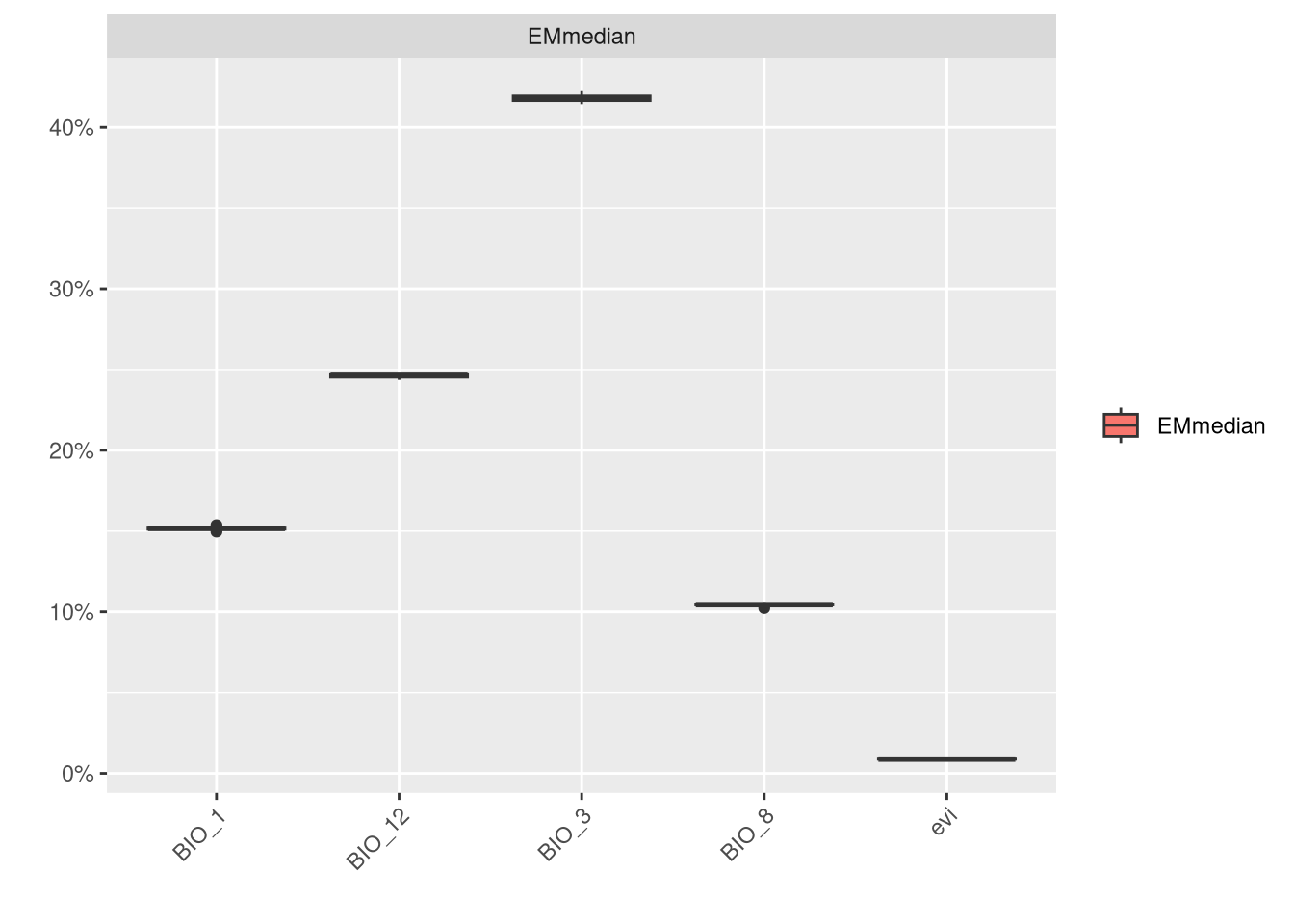
In this model, BIO_12 and BIO_7 are clearly the most important variables, while NDVI contributes the least to the models.”
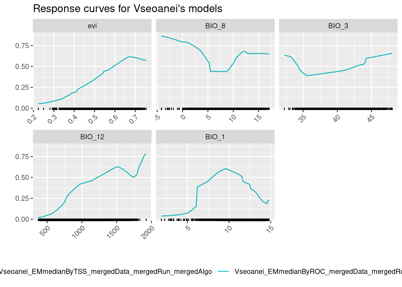
And finally we can check variable response curves.
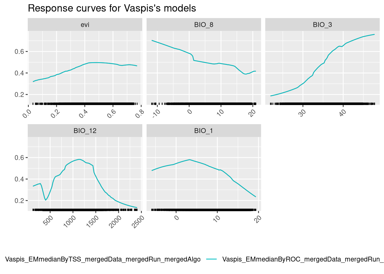
The ensembled models provide a single response curve for each variable, which is easier to interpret than before. We should give more importance to the BIO_12 and BIO_7 curves, as those are the variables that contribute more to the models. The model seems to increase the predictive probability with the increase of the value of these variables. Notice how the NDVI, which is the least important variable, appears to have a trend, but the prediction range associated with it is low.
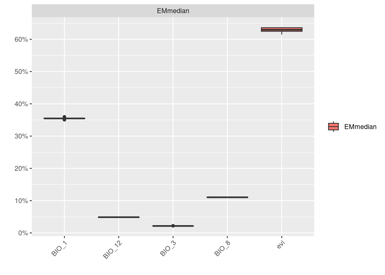
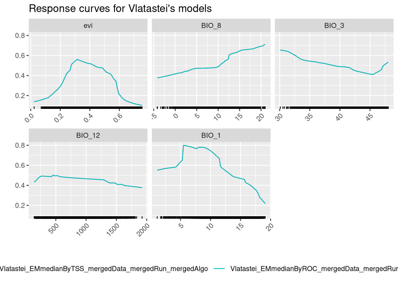
8.2 Ensembling Vipera latastei
Repeat the code, changing the model.
vlName <- load("models/Vlatastei/Vlatastei.EcoMod.models.out")
vlModel <- eval(str2lang(vlName))


# Ensemble
vlEnsbl <- BIOMOD_EnsembleModeling(bm.mod = vlModel,
                                   models.chosen = 'all',
                                   em.by = 'all',
                                   em.algo = 'EMmedian',
                                   metric.eval = c('TSS', 'ROC'),
                                   var.import = 3)


# Plotting examples
plt <- bm_PlotEvalBoxplot(vlEnsbl, group.by = c('algo', 'algo'))
8.3 Ensembling Vipera seoanei
And for the third species:
vsName <- load("models/Vseoanei/Vseoanei.EcoMod.models.out")
vsModel <- eval(str2lang(vsName))


# Ensemble
vsEnsbl <- BIOMOD_EnsembleModeling(bm.mod = vsModel,
                                   models.chosen = 'all',
                                   em.by = 'all',
                                   em.algo = 'EMmedian',
                                   metric.eval =  c('TSS', 'ROC'),
                                   var.import = 3)


# Plotting examples
plt <- bm_PlotEvalBoxplot(vsEnsbl, group.by = c('algo', 'algo'))