In this post, I’ll describe the process I used to create the Ptolemy 3D map. Although I have aimed this tutorial at a beginner level, it still hinges on GIS concepts. Thus, some knowledge of geospatial data manipulation and familiarity with the blender interface makes it easier to follow the instructions. All software I use for this tutorial is free, open-source, and works on most common operating systems.

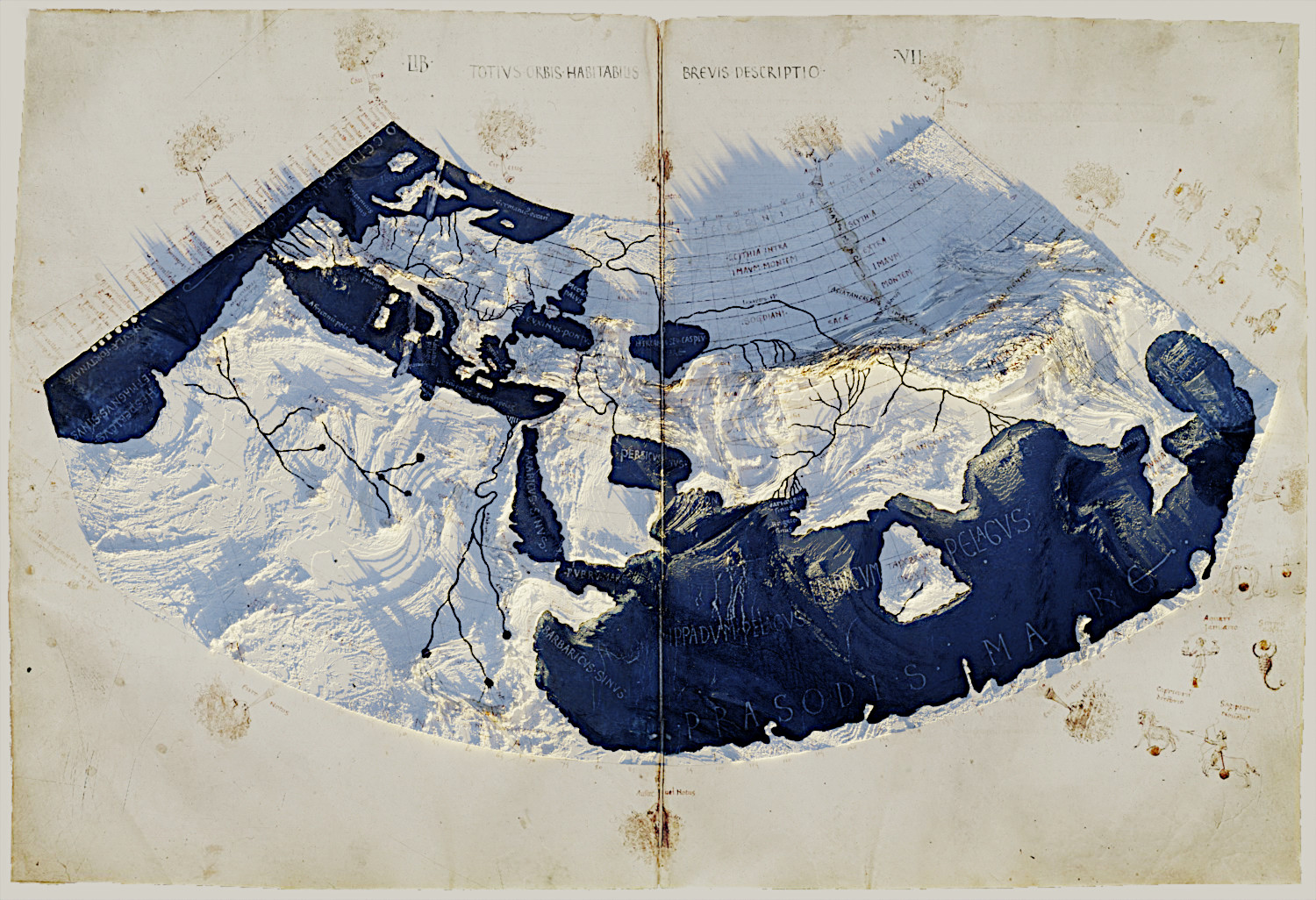
Here is the final image we will be creating.

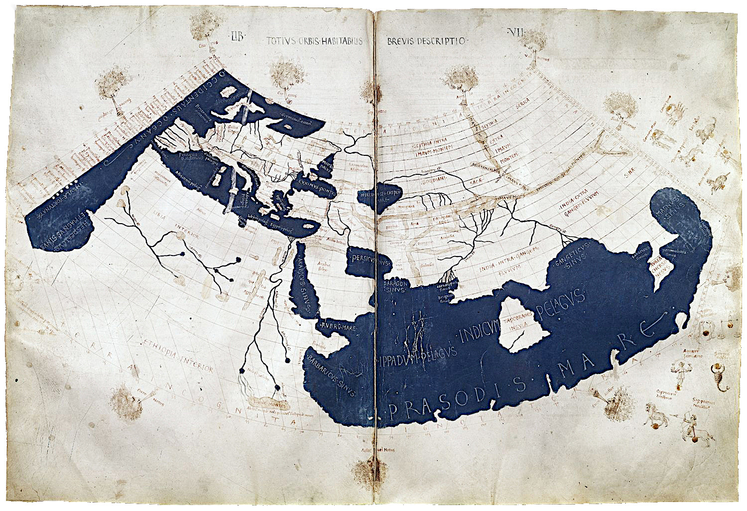
The source map for this project is based on Ptolemy’s work and depicts the Ecumene or the known world during the 2nd century. It was centered on the Mediterranean, showing the European and African coasts in great detail. It is curious how well known this coastal area was at the time, compared to Northern Europe. The map summarizes geographical knowledge during the Roman Empire. It does make some sense they have accumulated detailed knowledge here. However, the Romans had already settled in England by this time. Hence some geographical information was already available. The original map was part of Ptolemy’s Geographike Hyphegesis or Geographia manuscript. Unfortunately, no manuscript survived. This work is no less than extraordinary: it provided a table of features (cities, mountains, and others) with coordinates based on latitude and longitude, from western Europe to Asia, and a treatise on how to produce maps with a description of map projections. The map coordinate system relies on latitude measured in degrees from the equator. The prime meridian defining the origin for longitude is in the Fortunate Islands (Canary Islands). These islands were the most western point known at the time.

Ptolemy’s work was the most accurate and exhaustive atlas of its time, at least within the Roman world, influenced many cultures and set standards for cartography production. Although the manuscripts did not survive, many Latin and Arabic translations did. The map I use here is from the Jacobus Angelus’s Latin translation of Ptolemy’s work (1406 AD). The map was probably updated with new geographic features in this reedition and most certainly stimulated the creation of new maps. However, the known world to Europe did not change much until the 16th century.

Advertisement

Preparing the data

I use the base map found here for this tutorial. I have slightly edited the image in GIMP to remove the background and the clips in the corners. I also did a small crop to adjust to the extent and used some sharpening. This map will be used as a texture for the 3D object later. The final size of the image is 1500x1026px, which we will be using a lot to maintain the proportions of the images we will be creating. You can find my file here.

For elevation data, I have used the GEBCO dataset. It combines both elevation and bathymetry data we need to produce the 3D. I downloaded the global GeoTiff sub-ice data file that is divided into several tiles. I merged the necessary tiles to have the extent from -30° to 180° of longitude and -50° to 90° of latitude. Since the full resolution and extent available is excessive for this project, I cropped and scaled it down to more manageable file size. This can be done with QGIS or, if you have some command-line skills, at the terminal with GDAL. With QGIS, just open the images and use Raster->Miscellaneous->Merge tool to merge the tiles to a single image. This may take a while as the images are very large. Note that decreasing the resolution before merging might generate some edge effects on each tile due to the lack of needed information on the neighboring tiles. Crop with Raster->Extraction->Clip Raster by Extent and use -30,180,-50,90 in the extent field to reduce to the desired area of this project. Finally, you can reduce the resolution. For that I have used the Raster->Projections->Warp tool. I set the resolution to 0.01 which is only a decrease by a factor of about 2 but it was enough to keep the processing going smoothly on my computer. I had some problems with this tool because it was resetting the longitude extent to -180/180 and created a very large image. To avoid this, I have forced the options to have the same extent as the clipped layer. So I set the resampling method to average, the output resolution to 0.01 and for the georeferenced extents of the output file parameter I used the original layer by using the dots icon on the right of the field.

(De)georeferencing the map

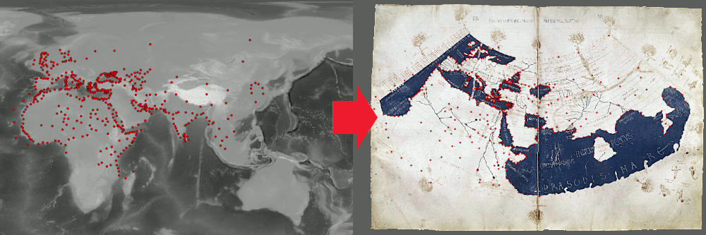
The objective here is to overlay the elevation data with Ptolemy’s projection as accurately as possible. This includes heavy distortion and twists of the elevation data to fit the real geographic features into the known world map of Ptolemy. We can’t rely on simple affine or polynomial transformation. We will have to use thin-plate splines that allow the level of distortion we need. However, we will have to reference a lot of points to be able to succeed in this. I have used the Raster->Georefencer tool in QGIS. Open the Ptolemy’s World map file in QGIS and the elevation model in the georeferencer tool. The intention is to create as many points as possible in the elevation map and give the corresponding point in Ptolemy’s World map. I have created 539 points around the identifiable features and, by trial and error, added/removed some to extend the elevation data over the whole map. I avoided point configurations that created heavy and visible stretches of the data, particularly on the bathymetry, that would affect the 3D. You can see the set of points I have used in the next figure and you can also download the file to directly import to your project. If you are using your edited image of Ptolemy’s map, this set of points might be shifted and you will have to create your own.

After creating all the necessary points, simply use the Thin Plate Spline option and save it to a new file. This map will serve as a displacement texture for the 3D in Blender. We won’t need any coordinates for the 3D but we need to make sure that the images overlay correctly with the World map. For that you can use Raster->Extraction->Clip By Extent tool again and set the extent to the Ptolemy’s World map to make sure it has the same proportions. Another thing that we need to get rid of is the elevation data… Blender does not read the numeric information associated with the pixel-like the GIS, only the color intensity. This means that we have to convert the map to a typical image without real elevation data but with different shades of gray proportional to the elevation. We first choose a gradient from black to white in the symbology (I’m using a linear gradient but you can play with the gradient to highlight some features). We now have to export the image to a typical image file using QGIS. We can use for this the menu Project->Import/Export->Export Map to Image. In the popup window use the layer to define the extent and choose also the resolution to export (I used 600 dpi for this example).

Advertisement

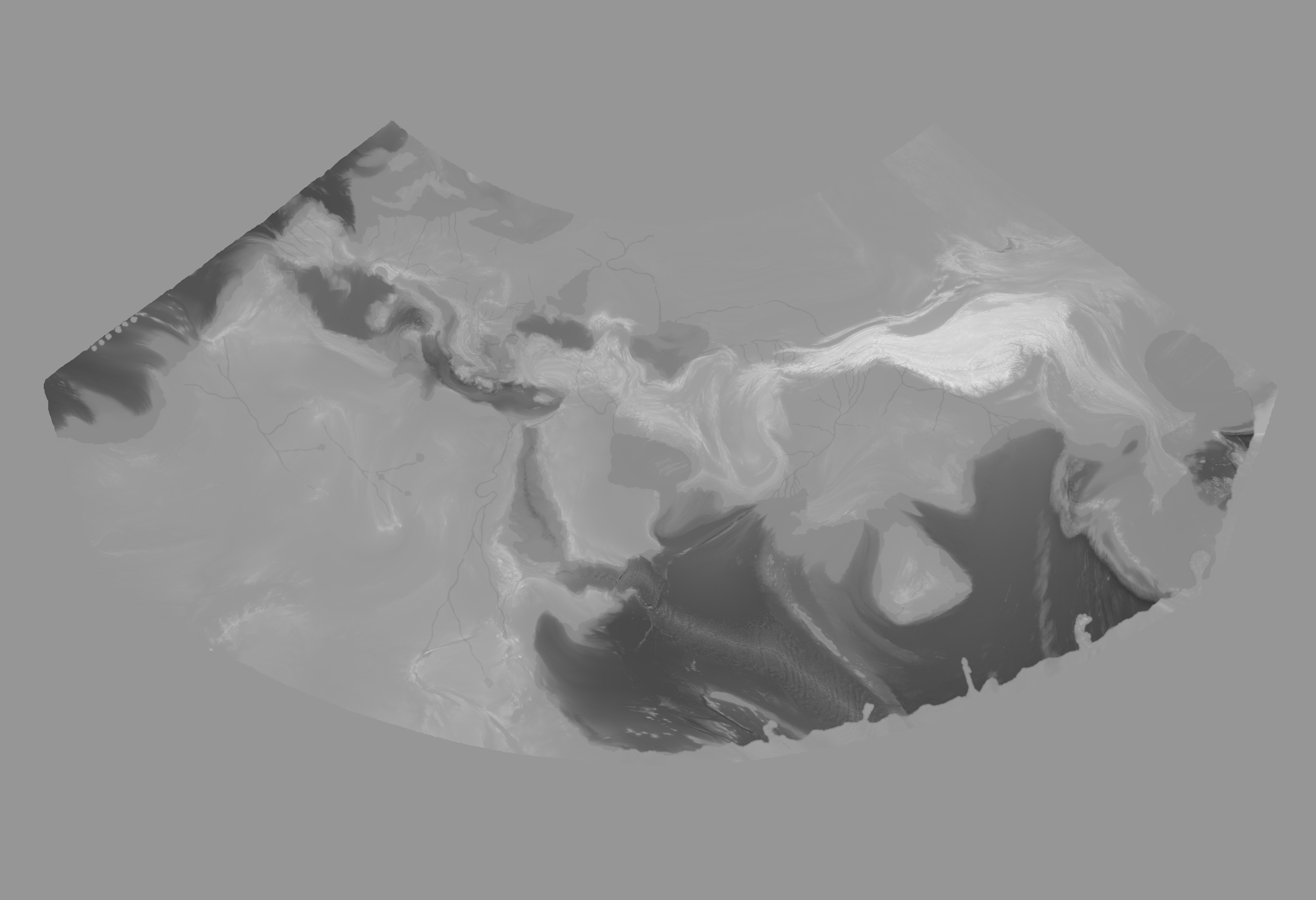
Prepare the elevation texture

With all the GIS work done, it is time to prepare textures for the 3D in a photo editing software. I have used GIMP, but you can use any other photo editing software (e.g. photoshop). The idea is to edit the elevation texture we produced above until it fits perfectly with Ptolemy’s map of the World. With the opened elevation image in GIMP, I added a new layer with Ptolemy’s map for guidance. Since it has a lower resolution, we need to scale it to the full extent of the elevation, and it should align with it. I created a few masks for the area where we should have elevation data and improvised on the southern part (Terra Incognita) and on the islands in the western area to create land elevation. I have used the clone tool for most of this task. You can check the layers I have produced to get the final elevation texture map in the animation below.

The animation highlight some of the details with arrows. There is a general land mask that was based on Ptolemy’s map to provide more detail and sharpen the land/water transitions, including the rivers. It is a land mask with rivers with a medium gray tone. I used the color pick on a known land area in the elevation map to select the gray intensity for the land mask. With all layers active, export it to a png file. You can find the file I produced here.

Make the 3D map

We have everything ready to go to Blender. Since we have all images with the same proportions, we can easily create the 3D scene. Just open Blender and erase everything in the default scene. Start by adding a plane and scale it to the image size. To avoid a large mesh delaying the viewport, I set the scale to 15 x 10.26 m. I edited the plane and added two vertical edges and a horizontal one. It promotes near-square subdivisions, resulting in a better 3D model. Then I moved to the modifiers panel, added a subdivision surface and set the subdivision algorithm to simple. This algorithm avoids smoothing the plane corners, maintaining the rectangular shape. To avoid a large mesh in the viewport, I use a lower number of subdivision iterations (around 8) for the viewport but set render iterations to a minimum of 10 to increase the detail in the final render. Next, I added a displace modifier that takes the elevation data and projects it to the mesh. Select a new image texture and open the file created above. You can tweak the displacement options (strength and mid-level) to find the best settings for you. Now the object needs the texture of Ptolemy’s map. In the texture panel, add a new texture, choose Image in the color selection and open the Ptolemy’s World map image. The object is done. We just have to create a camera and lights to render the scene.

In this project scene, I prefer an orthographic camera placed above the map. Setting the export resolution to the same size as the image allows adjusting perfectly the camera to the map. In the orthographic scale, set the value to 15 (or adjust if the dimensions you are using are different). For the light setting, I prefer to use an environment texture with an HDRI image. It makes it so easy to set excellent lighting for these maps. I have used the free and excellent Poly Haven to get this image. It creates dramatic shadows (perhaps a bit excessively…) and adds a warm tone to the map, which I like. In Blender, go to the World Proprieties panel, set the color to Environment Texture, and open this file.

You may now render the image (menu Render->Render Image or F12) and you should get a similar image to the one in the beginning of the post.

Advertisement

Final considerations

I prepared this tutorial so anyone can follow it, regardless of experience with the programs used. To achieve this, I have tried to simplify the entire process. For my original map, I have used other strategies that included some programming in Python/R, and I have extensively relied on the bash terminal for most of GIS and image exportation. This gave me good control of the maps and resolution. Also, I have used images with higher resolution to produce the final 3D. It was the maximum resolution that I could work on my desktop computer without excessive stalling and errors. However, if you follow this tutorial you will still be able to produce very high-quality maps!