Obtaining data from publicly accessible databases, cleaning it up, and creating 3D density maps has become quite popular lately. In this post, I will explore how to do this in R using simple and straightforward methods and packages. Most of the heavy coding is already done in these packages, so we’ll be producing the glue code around them to produce a 3D map from scratch (Disclaimer: there will be some rant about the pipe in R as well…)

As a quick overview, we will be collecting observation data for the common raven (Corvus corax) from the Global Biodiversity Information Facility, cleaning the data and using it to generate gridded density maps.

Advertisement

Setting the scene

We will be using some packages for this script:

• rgbif to search and download observation data from GBIF
• CoordinateCleaner to clean up geographical data
• spatstat for easy Kernel density calculation
• terra, which replaces raster package for working with spatial rasters and vectors
• rayshader does the 3D magic in R.

Most of these packages can be installed via CRAN using the typical install.packages("xxxxx") command. However, I encountered some errors with the CRAN version of rayshader and had to install the development version instead. To do this, you will need the devtools package and run the command devtools::install_github("tylermorganwall/rayshader").

library(rgbif)
library(CoordinateCleaner)
library(spatstat)
library(terra)
library(rayshader)

Obtaining the data

We will be searching for all available data on the common raven (Corvus corax) at GBIF. While the GBIF web interface allows users to select and download a zip file, we will be performing all of these tasks directly from R. To begin, you will need to create a GBIF account if you haven’t already done so. To register, visit their webpage and create an account.

Once registered, we set some variables with our GBIF credentials to establish a connection:

user <- "xxxxxxxx"
pwd <- "xxxxxxx"
email <- "yyyy@xx.zz"

To search for data, we will need to use the taxon key for Corvus corax rather than its name. To retrieve the taxon key, we can use the taxa database provided by GBIF.

tx <- name_backbone_checklist("Corvus corax")
txkey <- tx$usageKey

We can now query the GBIF database for observational data. To retrieve only observations with latitude and longitude, we will set two filters: one for the taxon and one for the presence of coordinates. In this example, we will use the comma-separated values (CSV) format. Please note that this process can take some time, as there are many lines of data for this species. To monitor the download status, we can set a download wait flag and check for the status change from ‘running’ to ‘succeeded’ before downloading the data.

cc <- occ_download(
    pred("taxonKey", txkey),
    pred("hasCoordinate", TRUE),
    format = "SIMPLE_CSV",
    user=user,pwd=pwd,email=email)

res <- occ_download_wait(cc)
data_file <- occ_download_get(cc)

The occ_download_get will download a zip file to the current working directory. We can import the data to a tibble:

d <- occ_download_import(dataFile)

If we need to use the same data in another R session or script, we can avoid querying the GBIF website again by using the zip file that was saved. To load the data from the zip file, we can use the following command, replacing GBIF_data.zip with the actual name of the zip file:

d <- occ_download_import(as.download("GBIF_data.zip"))

Coordinate cleaning

Instead of using the whole dataset blindly, we will clean some of the observations based on the attribute data. The CoordinateCleaner package facilitates this task by providing a set of methods to remove unnecessary data. We convert the tibble to a data frame and flag each record based on a set of criteria, including coordinate validity, identical coordinates, erroneous coordinates, and observations that match known geographical locations such as capitals, country centroids, or institutional headquarters.

dat <- data.frame(d)
tests <- c("capitals", "centroids", "equal", "gbif",
          "institutions", "zeros")
flags <- clean_coordinates(x = dat,
                           lon = "decimalLongitude",
                           lat = "decimalLatitude",
                           species = "species",
                           countries = "countryCode",
                           country_refcol = "iso_a2",
                           tests = tests)

A few proportion of records (67753 out of 7606191) match the criteria and are flagged for removal (note that GBIF is constantly adding more data and your dataset might have different size). We can inspect them further to verify if they are indeed erroneous. For this example, we will remove all of them from the dataset without checking.

dat_cl <- dat[flags$.summary,]

We may still have some data that needs to be removed. For example, we can use the coordinate uncertainty attribute to eliminate points that are georeferenced with high uncertainty. We can achieve this by applying a filter that keeps only records with uncertainty values of 10 km or lower, or records without uncertainty information (using the is.na() command and the OR operator, the vertical bar).

crd.u <- dat_cl$coordinateUncertaintyInMeters
dat_cl <- dat_cl[crd.u <= 10000 | is.na(crd.u),]

GBIF provides plenty of information for each record. We can also removed those records that are known to be fossils:

dat_cl <- dat_cl[dat_cl$basisOfRecord != "FOSSIL_SPECIMEN",]

We can also remove those records that do not have any individual count, keeping all those that have at least one. Similarly to what we did before, we also need to retain all those that do not have any information for the individual count.

ind.count <- dat_cl$individualCount 
dat_cl <- dat_cl[ind.count > 0 | is.na(ind.count) , ]

As a last step, we will remove older records using an arbitarly chosen year of 1970. Again, we want to keep records that do not have this information as well.

As a final data cleaning step, we will remove records that are older. We will remove all records that have a year of observation prior to 1970. However, we want to keep records that do not have a year of observation specified.

dat_cl <- dat_cl[dat_cl$year > 1970 | is.na(dat_cl$year), ]

As we only need the coordinates, we will extract the longitude and latitude and create a new data frame with x and y columns. We can still perform further cleaning by assuming that all data is a single observation. This allows to remove duplicated coordinates arising, for instance, from observation on different years.

crds <- data.frame(x=dat_cl$decimalLongitude, y=dat_cl$decimalLatitude)
crds <- unique(crds)

With this last step, we retained about 18.8% of the original dataset.

Advertisement

Estimating densities with kernel

Kernel density is a non-parametric way to estimate densities from data. Using the coordinates, we can estimate densities over space, following to the local number of observations and, thus, showing the distribution of the data.

The kernel density estimator works by setting a distance (the bandwidth) for each point to estimate the contributions of all points to a specific location. With that it is able to estimate a density to that target locations, affected by all the points within the chosen distance. The larger the distance, the larger will be the smoothing effect.

We use the package spatstat to estimate the kernel density. It has it own object class “ppp” for the input point pattern. Thus, we have to convert the coordinates data frame into a ‘ppp’ object. For that we need the coordinates x and y and an extent.

p <- ppp(crds$x, crds$y, c(-180, 180), c(-90,90))

The density is estimated over a gridded surface. Similarly to a raster, we have to define the resolution. Here I’m using 3600 columns and 1800 rows, which, given the extent, translates to a spatial resolution of 0.1 degrees. Of course, the higher the resolution, the more time is needed to finish all the remaining tasks, and the higher processing burden. I’m using this value for the bandwidth distance (the sigma parameter in the function).

ncol <- 3600
nrow <- 1800
d <- density(p, sigma=0.1, dimyx=c(nrow, ncol))

We do a fast plot to check the density estimation. I prefer to visualize the logarithm of the densities plus 1, to better visualize the distribution.

plot(log1p(d))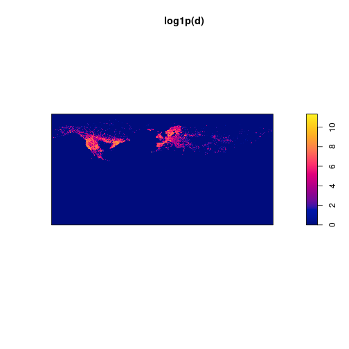

Plotting in 3D

We are using the rayshader package to plot the 3D densities within R. There are some conversions of data to matrix format which need some rotation of the matrix to orient correctly the data. It is pretty straightforward.

First we convert the density estimation to a matrix with (nrow, ncol) size. However, to correctly display it, with need to rotate it to (ncol, nrow). This is a 90 degree clockwise rotation that we can accomplish with a small trick: just flip the matrix vertically and translate it. Afterwards, we eliminate all smaller values (<1).

mat <- as.matrix(d)
mat <- t(mat[nrow:1,])
mat[mat<1] <- 0

The matrix mat has the information of the densities. To get a better plot, having some information about the land masses would be useful, especially to rapidly locate the density peaks. The rayshader package allows to overlay textures and multiple 3D objects but this, in my point of view, complicates the code to get a nice looking 3D map. The way I decided to explain here requires a single matrix with all the information for the height. This includes a bottom height to oceans, a slightly higher value for land masses and then the density estimation. Thus, a pixel will get a very low value (-1000) if it is ocean, a zero value if it is land, and a positive value if has some density.

So, let’s get some information about land masses for the planet. I have used the countries data from Natural Earth. We don’t really need the countries, but the polygons do represent well the land area. We will use the terra package to read the vector data and to rasterize it to a similar grid as the densities. To do this, we use the same resolution (3600 columns and 1800 rows) for the rasterization process. We convert the reuslting rater to matrix and this will be our basemat. As said before, the land will have a value of zero, so we multiply the matrix by zero. All other pixels will be set to NA, which are the ocean pixels.

To align with the densities matrix, we have to transpose the resulting matrix. This way, the equivalent pixels in both matrices represent the same geographical area.

world <- vect("ne_10m_admin_0_countries.shp")
baserst <- rasterize(world, rast(ncols=ncol, nrows=nrow))
basemat <- as.matrix(baserst, T) * 0
basemat <- t(basemat)

Now we have to mix both matrices to produce a single one with the height information for the 3D plot. So, 1) we make sure that all pixels with density outside land area receive the same base value. This will avoid sharp changes in peak values and associated 3D artifacts. We can use the density matrix to filter the basematrix and find these values. 2) we guarantee that all ocean pixels receive a very low value (-1000) to give an impression of height to land areas. Finally, 3) we sum both matrices to get the final height matrix. Summing the density matrix will only change pixels with zero value to the density value. Because we eliminated all densities lower than 1, the minimum density height is 1.

basemat[mat > 0] <- 0
basemat[is.na(basemat)] <- -1000
mat3D <- mat + basemat

We have now to prepare a gradient of colors to illustrate the height. I’m using the palette SunsetDark reversed, with 256 gradient steps. This will give a nice light to dark color gradient and rayshader will take care of associating each color to the height map.

hcolors <- rev(hcl.colors(256, palette="SunsetDark"))

We can now produce a 3D plot. This requires a two-step process: first, we produce a low-quality image, and then we use those settings to render the plot in high quality.

Most of the code about rayshader uses the pipe in R. I will also use it here but before we move on, I’d like to share my personal opinion on the pipe in R (the promised rant). I have some reservations about it. While the idea of data flowing in a pipeline it is interesting, I think it can also make the code less readable and harder to debug, particularly when the code becomes more complex and bigger. An many times, slower. Additionally, it can be confusing for beginners who are still learning base R as they still have to start there. It seems to create the need to learn almost two different languages… In my opinion, if you don’t want your code flooded with ephemeral transient variables, it’s often better to encapsulate the code in simple functions rather than relying too heavily on the pipe. R will take care of eliminating non needed variables as needed. It seems a way to avoid learning how to write better code, rather than to facilitate script writing. To be clear, I believe pipes have their place, like in the bash terminal where I use them constantly and can be extremely useful. But not in R!!!

Moving on, we need to set now a 3d scene. The variable I’m passing to the pipeline is the logarithm+1 of the height matrix. This information is used to set up the colors in the 3D scene, but the real height is given afterwards, with the heightmap argument for the plot_3d function. Before, the function height_shade relates the data in the pipeline to the color gradient, producing a texture to the 3D scene. Note that by using the logarithm, all negative numbers are set to NA, so they don’t receive any color.

For the plot_3d function we can also set a series of other parameters. I’m seting the zscale to rescale the densities height by a factor of 100, so they don’t step out of the camera view. I’m setting the theta, phi and zoom parameters, which are placing and orienting the camera, by setting an angle of 0, a height of 50 and a zoom allowing to see the whole map. The window size parameter sets the dimensions of the image to be created in pixels, which corresponds to an HD resolution here (1920x1080).

There are also some shadow parameters for the general scene. Because we are using a matrix that defines the whole world extent, the shadow is show for the rectangle of the world. It is not mandatory, but the map looks a bit better if is defined. I set the shadow to a a depth a bit lower than the minimum height value in the matrix.

log1p(mat3D) |>
  height_shade(texture = hcolors) |>
  plot_3d(heightmap = mat3D, 
          zscale = 100,
          shadowdepth=-1050,
          solid = TRUE,
          soliddepth = -1050,
          theta = 0,
          phi = 50, 
          zoom = 0.5, 
          windowsize = c(1920, 1080)) 

Advertisement

With the low quality scene produced, we can now export it to a file with high quality using the render_highquality function. We need to set a few parameters, though. The filename parameter defines the name of the image to be exported. The quality parameters are the number of samples, which determines the number of samples for each pixel, and max_depth, which defines the maximum number of bounces that a light path can make in the scene. Higher values for these parameters result in better quality but take longer to render. We also need to set the light source parameters. The direction is 35 degrees clockwise from North, with an altitude of 60 and intensity of 750. There are many other parameters that can be fine-tuned to customize the final image. However, for simplicity, these settings already produce a nice-looking map. Since we have already defined the camera in the previous step and only want to export the image, we can set the interactivity to false.

render_highquality(
    filename = "DensityMap.png",
    samples = 200,
    max_depth = 150,
    lightdirection = 35,
    lightaltitude = 60,
    lightintensity = 750,
    interactive = FALSE
)

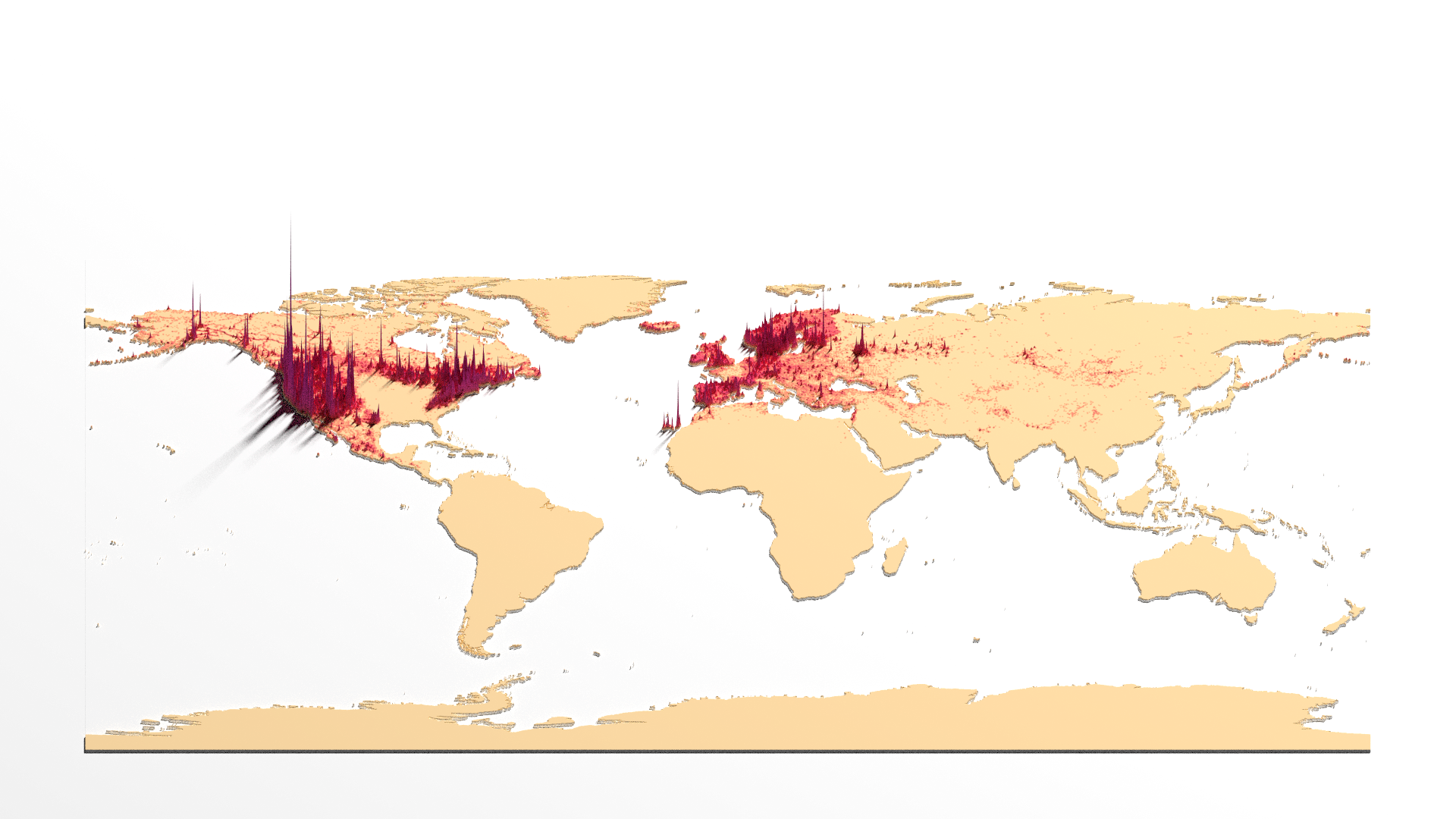
And that’s it: a simple way to produce a density 3D plot from data collection and processing, to spatial density calculation and 3D rendering a scene. Of course, many post-editing is required for this image, like adding title and data sources, etc.

You can explore a bit further to produce high quality 3D maps. The rayshader website has plenty of tutorials from the author of the package on how to do that, including animating the camera and light sources, overlaying images to 3D scenes and others. There plenty of resources in the internet on how to use rgbif package and how to perform coordinate cleaning with the packages we have used here.