Georeferencing data from a digitized map in R
A crucial step we often face in a beginning of a study is data gathering. We either go to the field, dig into museum’s collections, search literature, navigate databases or follow any other strategy. Very often important spatial biological data is stored only in maps. Either a distribution of a species, some sampling locations were shown in a map but no coordinates given, some old distribution map that would help to complete some temporal analysis of a distribution, etc. These data are extremely valuable for research and often we find ourselves in the process of digitizing maps, georeferencing and painfully extract the data we need from the map.
A few years ago I was immersed in a one of such tasks. I decided to write a few scripts to assist on the processes of georeferencing and extract data. Later I packaged the scripts in an easy to use R package named speciesdigitizer.
Advertisement
Installation
The easiest way to install package is probably using ‘devtools’:
library(devtools)
install_github("ptarroso/speciesdigitizer", subdir="source")
The package has a few dependencies on other packages, so if you don’t have them already installed, ‘devtools’ will prompt you for authorization. The dependencies are
- ‘tcltk’: likely already installed and is provides access to the graphical interface toolkit.
- ‘sp’: a very common package to work with spatial data
- ‘rgdal’: link to GDAL library and provides access to many spatial data file formats
- ‘vec2dtransf’: provides the 2d coordinate transformation for georeferencing
If you prefer, that is also a built package file that you can download and install from file in your R session.
Using the package
The speciesdigitizer only uses affine transformations. This means that the image to be georeferenced must only require simple transformations to align to the coordinate system of the map. Typically these simple transformations include translation, rotation and scaling. Complex distortions (quadratic, splines, etc) are not supported.
To illustrate how to use the package, I’m using an example page of the Distribution Atlas of European butterflies that you can view here. This is one of the first images I found after googling with the keywords “Distribution atlas”…
You only need two commands to start georeferencing and extract data: open the library and open the graphical interface (GUI):
library(speciesdigitizer)
speciesdigitizer()
The GUI should appear and look like this:
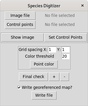
We need two files in the computer: an image to be georeferenced and a set of control points with real coordinates of locations easy to spot in the map image. If a file named “ControlPoints.txt” is found in the same path as the image, then it is automatically added, otherwise you have to open it with the respective button. This file should have two columns with X and Y coordinates (in this order) and at least four points necessary to calculate the transformation. In this example I’m using of four control points that have the coordinates of the grid intersections that are nearest to the corners. The order will matter later, so this points are in clockwise order, from the top left. The “ControlPoints.txt” looks like this (field separator in the text file must be a semicolon “;”):
| X | ; | Y |
| -10 | ; | 60 |
| 40 | ; | 70 |
| 40 | ; | 35 |
| -10 | ; | 35 |
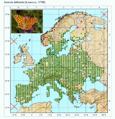
After opening the image and respective control points, we have to locate in the image the respective control points. The process is simple: press show image button and adjust the size of the image to make easier to locate points. When ready, press “set control points” and locate the points in the image with the same order as they are in the control points file.
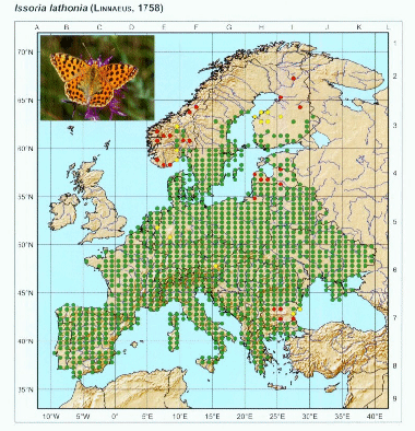
You can repeat this process as many times as needed to get a good position of the red markers that appear after setting the last point. This will give the necessary information to transform the image to align to the coordinate system. Once ready, we can set the grid spacing on X and Y directions. In the image, we can notice that there are 5 points per 5 degrees of longitude, which means that there is 1 point/degree, thus we set X spacing to 1. On the other axis, there are 10 points within 5 degrees of latitude, which means 1 point per 30 arcmin or 0.5 degrees. We set Y spacing to 0.5.
We are now set to georeference the points. This can be done automatically by using the color of the points, thus only images that have contrasting colors for points in relation to the rest of the elements of the map will work. However we can adjust a color threshold, so other elements with similar color are filtered out. So press “point color” button and select one of the points in the map.
Again, you can repeat this process as many times as needed to get a good selection of points. You can adjust the threshold and select different points to get different nuances of the color.
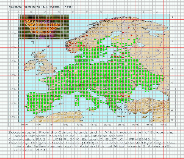
With the final check we can view the georeferenced map with a grid with the corresponding spacing and the points that we were able to detect. We can use this process to first check the grid alignment and make the necessary adjustments on the location of control points or the grid spacing. Than we can check the detected points.
Some maps have less contrast between points and other map elements, so some tweaking here might be needed. So, you have the + and - buttons to add or remove points from the image. Once you press the button you can locate the points to add (or remove) in the map with the left mouse button. Once done, press the right mouse button and the points will be plotted (or removed). Of course, you can directly skip the automatic detection of points and add them manually. In this step, the points are adjusted to the grid, thus every point you add to the map are with exact coordinates of the centroid. This can be useful with, for example, old black and white maps.
After checking you can export the points to a text file with the last button. If you check the box “Write a georeferrenced map”, than, along with the points, a geoTiff with the georeferenced map will be saved along the points. Note that this raster is created by adjusting the transformed pixel coordinates to the nearest grid. The grid is based on the average x and y resolution taking to account the original number of pixels in the image. You can open both map and points in a GIS and check for errors.
Advertisement
Other example
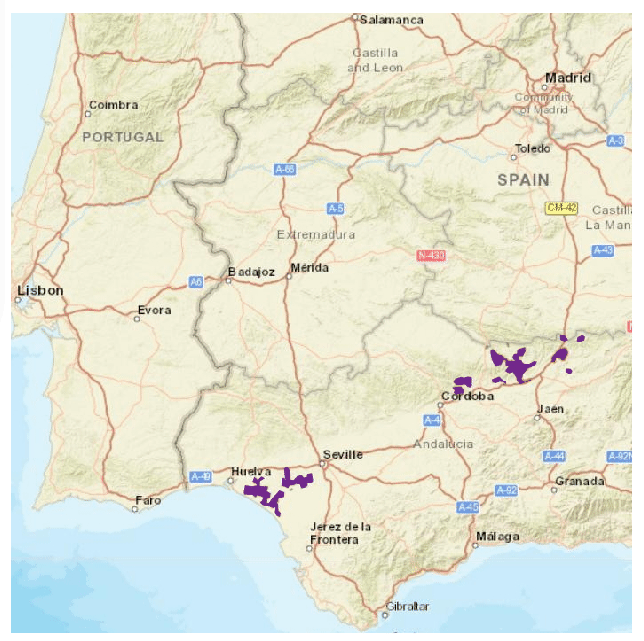
The speciesdigitizer() only georeferences points. However, this does not mean that it can be useful with other shapes of spatial data. For instance, it can map a distribution of points within a colored polygon in a map. This might be useful to get distribution data as points but also to later apply some geoprocessing to derive a polygon from the set of points. Let’s see this with an example map with the Iberian lynx distribution. The color of the polygon contrasts with the background map so it should be fairly simple to extract. I’ll use this set of control points:
| x | y | city |
| -9.150019 | 38.725267 | Lisbon |
| -6.333333 | 38.9 | Mérida |
| -3.716667 | 40.416667 | Madrid |
| -3.600833 | 37.178056 | Granada |
| -5.351667 | 36.131667 | Gibraltar |
| -7.916667 | 37.033333 | Faro |
As you see I have an extra column in the control points that will be ignored by speciesdigitizer() but helps me remember the order of points to locate on the map. The process is the same as before: set control points, define a grid spacing, do a final check and export. Here I use a very small grid (0.01 degrees on X and Y) to capture the distribution of the polygon.
There is, however, a limitation to the minimum grid size. The package does not perform any interpolation of the values which makes the minimum grid spacing dependent on the original resolution of the map. If you need more resolution, than you should increase the size of the image in an appropriate software like GIMP, photoshop or any other image manipulation software.
Some concluding remarks
The speciesdigitizer started as a few scripts that helped me to automate the process of digitizing data. As I began to realize that this automation was of the interest of others, I decided to package the scripts so it could be easily distributed and installed. The package does work but it was not tested to exhaustion with many different maps. Thus, if you find it useful and have suggestions, comments or you found some bug, please let me know by opening an issue or by any other contact you find in this page.