This is the last post of a series of 3 dedicated to phylin. The idea was to show different uses of phylin that would go beyond the typical application of the method as detailed in the publications. This time I will be using a Jaccard distance matrix instead of a typical genetic distance matrix with phylin. This will allow to map a contact zone without recurring to habitat or niche modeling.

Some background

In the previous posts and in the examples given in the two articles we used a genetic distance matrix with phylin. This follows our original intention with the method that was related to mapping genetic differentiation with only a genetic distance matrix and spatial locations as input. Later we allowed different models of spatial isolation to interact with the method. But… Could we use other metric of differentiation rather than genetic?

The Jaccard index measures the similarity between two sets by relating the elements that are common to both sets to the total elements. A value between 0 and 1 is obtained indicating low to high similarity. The Jaccard distance measures the dissimilarity between the sets. It is the complement of the index (1 - Jaccard index), thus, low values indicate high similarity.

The idea behind this example is to analyze the possible extent of the area where two species co-occur. The data we will be needing are the precise observations of each species. As in the previous threads in this topic, we will simulate some data.

Needed packages

In this example we will be using two other packages along with the last version of phylin. We will need the package raster that complements well the phylin for displaying and raster calculation purposes and the package philentropy that provides functions to calculate multiple similarity metrics.

library(phylin)
library(raster)
library(philentropy)

set.seed(12)

I’ve also set the seed so you should get the same results as shown here.

Advertisement

Simulated data

We need to simulate the presence locations for two species that share a contact zone. We will randomly generate 50 coordinate pairs for each species based on the normal distribution. The first species is on the left side, so the mean X value is -500 and for the second species is +500. A standard deviation of 500 will generate enough spread for both species to contact around the horizontal middle of the extent.

sp1 <- data.frame(x=rnorm(50, -500, 500),
                  y=rnorm(50, 0, 500),
                  sp="sp1")
sp2 <- data.frame(x=rnorm(50, +500, 500),
                  y=rnorm(50, 0, 500),
                  sp="sp2")
sp <- rbind(sp1, sp2)

We are defining our study area based on the extreme locations of the species. For that, we will create a raster defining the study area with a spatial resolution of 100. Maybe it makes more sense with spatial units, so, let’s say that our unit of choice is the meter. It makes the pixel in our raster represent a square with a 100m side. The spatial resolution is important as should be carefully chosen as it is defining the area of sampling: if two observations of different species are in the same pixel, than we define it as sympatric.

To create the rasters we need to provide an extent and some values to store. The extent, as said, is defined by the min/max coordinate values plus an offset to add an extra pixel around. The values we provide are sequential integers, so they also serve the purpose of identification each pixel.

res <- 100
rst <- raster(xmn=min(sp$x)-res, xmx=max(sp$x)+res,
              ymn=min(sp$y)-res, ymx=max(sp$y)+res,
              resolution=res)
rst[] <- 1:length(rst)

So, let’s plot the data to get a better idea of our system.

plot(rst)
points(sp$x, sp$y, pch=ifelse(sp$sp == "sp1", 1, 2))
legend("topright", pch=1:2, legend=c("sp1", "sp2"))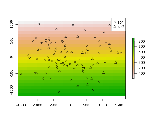

Distance matrices

We have now to produce the distance matrices. In this example will be using Jaccard distance instead of the genetic distance. We need to compare species composition in one pixel against another and do this for all pairs of pixels with species data.

sp$sites <- extract(rst, sp[,1:2])
occ.sp <- xtabs( ~ sites + sp, sp) > 0
jac.dist <- distance(occ.sp, method="jaccard")
dimnames(jac.dist) <- list(rownames(occ.sp), rownames(occ.sp))

Let’s see with some detail the above chunk of code. First we extract pixel data at each species location. Remember that when we created the raster we gave a different integer to each pixel, allowing pixel identification. In the newly created sites column in the sp data frame we store the information about in which pixel the presence resides, by extracting it from the raster with the species coordinates. With a bit of xtabs sorcery, we transform the previous data frame into a logical two-column table indicating if a species is present or absent in each pixel (with at least one presence of a species). In occ.sp, rows are pixels and columns are species. This is exactly the composition table that the Jaccard method needs for calculating the dissimilarity. To keep track of pixel sites, we give the same names to both dimensions of the resulting matrix in the last line.

The matrix of geographical distances needs to have the same format as the Jaccard distance matrix. This means that geographical distances are calculated between site locations (pixels) rather than between observations.

sites.crd <- coordinates(rst)[as.integer(rownames(jac.dist)),]
rownames(sites.crd) <- rownames(jac.dist)
geo.dist <- as.matrix(dist(sites.crd))

The trick I’m using here to get the coordinates is not very beautiful, but it does do work well here to maintain the same order as in the Jaccard matrix. I’m using the rownames, which are strings, converting them to integers and then use it to extract the needed coordinates by index. Geographical distances are calculated as the Euclidean distance between pixels.

Advertisement

Variogram and interpolation

We use both distance matrices as an input to build the variogram and fit a model.

gv <- gen.variogram(geo.dist, jac.dist, lag=50)
gv <- gv.model(gv, range=3000, sill=0.5)
plot(gv)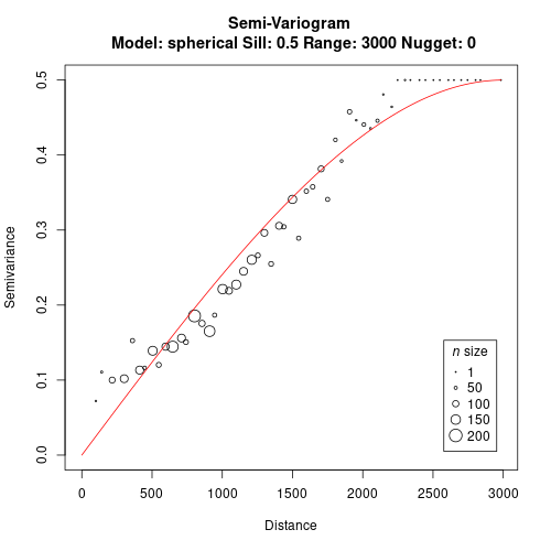

We can now use the model to interpolate over the space. The gridded data for the krig function is a table of coordinates of target locations to predict. We can use our previously created raster and extract the cell coordinates to a data frame. Than we can proceed to the interpolation of the likely area of occurrence of each species.

grd <- coordinates(rst)

i1 <- krig(sp$sp == "sp1", sp[,1:2], grd, gv, neg.weights=FALSE)
i2 <- krig(sp$sp == "sp2", sp[,1:2], grd, gv, neg.weights=FALSE)

As we are working with a gridded data set, for easy manipulation and plotting we can convert the interpolation predictions to a raster object. We use our study area raster as a template for two new rasters that are going to be filled with the interpolation predictions. Notice that this works because we extracted coordinates from the raster to define the interpolation area and it keeps the same order.

rst1 <- rst2 <- rst
rst1[] <- i1$Z
rst2[] <- i2$Z

We can plot both species predictions.

layout(matrix(1:2, 1,2))
plot(rst1, main="species 1")
plot(rst2, main="species 2", legend=F)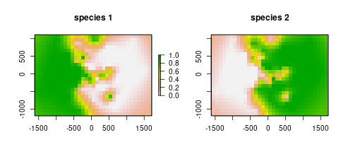

The models are depicting well the occurrence of the species. They are mostly the complement of the other, as we are only using two species. However, our objective here was to map a probable contact zone. Each of the rasters stores values for the probability of occurrence of the respective species. The product of the rasters will indicate the area where co-occurrence is most likely, thus we get the contact zone.

plot(rst1*rst2)
points(sp$x, sp$y, pch=ifelse(sp$sp == "sp1", 1, 2))
legend("topright", pch=1:2, legend=c("sp1", "sp2"))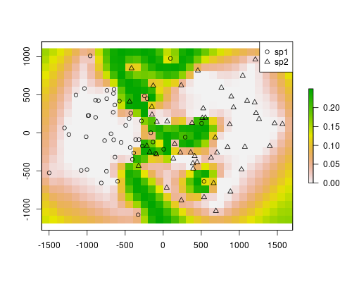

The contact zone is well defined in this example. However, this method will always define a contact zone, even if it doesn’t occur. For instance, if there was a barrier, the method would still predict a highly probable area for both species. This is the result of using only spatial locations and distances. In the map above, on the edges, a similar effect is visible. The value are quite high there because there are no samples (similarly, there would not be samples in a barrier). If you check the individual models above, you will see that the predictions for species 1 on the species 2 range are near zero, except in the edges, where the model lack information. However, because the contact area has higher values than the rest, it is still easy to find a threshold in this map that would highlight the contact zone, ignoring the other effects.

Advertisement

Conclusion

We manage to map the contact zone only with observations and independently of the niche requirements of each species. You can try to include the concept of resistance (see previous post) to better inform the model of the possible species movement and, thus, better distinguish between contact zone or barrier, for instance.

This ends this series of 3 post dedicated to different uses of the phylin method.